Making use of Bioconductor
Overview
Teaching: 180 min
Exercises: 120 minQuestions
How can I use Bioconductor packages in my project?
Objectives
Installation of Bioconductor packages
Understanding IRanges
Understanding GRanges
Loading up fastq files into R, ShortRead
Aligning reads using Biostrings
Plotting using ggbio
Bioconductor
Bioconductor is an open source, open development software project to provide tools for the analysis and comprehension of high-throughput genomic data. Bioconductor is similar to CRAN as an interface to access R packages, but contains packages that are more biology oriented and curated by the team of experts.
As bioinformaticians you will most likely operate within Bioconductor universe. It is designed with interchangeability in mind, many packages work together and creation of power-full pipelines becomes possible.
To install Bioconductor visit this page or do:
if (!requireNamespace("BiocManager", quietly = TRUE))
    install.packages("BiocManager")
BiocManager::install()
Lets install packages that will be useful in this lesson.
BiocManager::install(c("IRanges", "GenomicRanges", "ShortRead", "Biostrings", "ggbio", "biovizBase"))
Take a look how Bioconductor core packages are structured below. We will go through some of these packages. If you open any of these packages in the Bioconductor website, you can find there vignettes explaining in detail how to use them.
                   VariantAnnotation                Annotate variants, predict coding outcomes.
                           |
                           v
                    GenomicFeatures                 Making and manipulating annotations.
                           |
                           v
                       BSgenome                     Representation of full genomes and their SNPs.
                           |
                           v
                      rtracklayer                   Manipulating annotation tracks eg.BED, GFF, BigWig.
                           |
                           v
                    GenomicAlignments               Manipulation of short genomic alignments.
                      |           |
                      v           v
     SummarizedExperiment   Rsamtools  ShortRead    Load, contain and manipulate different data types.
                  |         |      |      |
                  v         v      v      v
                GenomicRanges     Biostrings        Lower level representations of short sequences.
                        |          |
                        v          v
               GenomeInfoDb   (XVector)             Utilities for genomic coordinates.
                        |     |
                        v     v
                        IRanges                     Representation of ranged data.
                           |
                           v
                      (S4Vectors)                   S4 implementation of vectors and lists.
IRanges
IRanges package designed to represent sequences, ranges representing indices along those sequences, and data related to those ranges. IRanges are very fast and provide multiple useful function to operate on them.
library(IRanges)
ir <- IRanges(c(1, 5, 14, 15, 19, 34, 40), width = c(12, 6, 6, 15, 6, 2, 7))
ir
IRanges object with 7 ranges and 0 metadata columns:
          start       end     width
      <integer> <integer> <integer>
  [1]         1        12        12
  [2]         5        10         6
  [3]        14        19         6
  [4]        15        29        15
  [5]        19        24         6
  [6]        34        35         2
  [7]        40        46         7
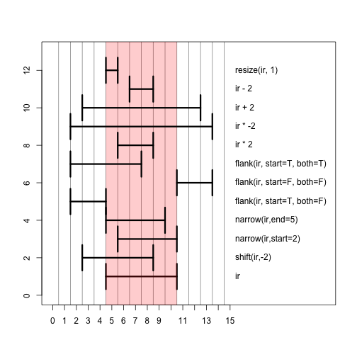
Lets use function below to plot our ranges. Notice widths, are they what you would expect?
plotRanges <- function(x) {
  height <- 1
  sep <- 0.5
  xlim <- c(min(start(x)), max(end(x)))
  bins <- disjointBins(IRanges(start(x), end(x) + 1))
  plot.new()
  plot.window(xlim, c(0, max(bins)*(height + sep)))
  ybottom <- bins * (sep + height) - height
  rect(start(x) - 0.5, ybottom, end(x) + 0.5, ybottom + height)
  axis(1)
}
plotRanges(ir)

Challenge 1
Create same plot as in plotRanges, but using ggplot2. How similar looking plot you can make?
Hint: Use
geom_rect.Solution to challenge 1
plotRanges_gg <- function(x) {
  bins <- disjointBins(IRanges(start(ir), end(ir) + 1))
  dat <- cbind(as.data.frame(ir), bin = bins)
  ggplot2::ggplot(dat) +
    ggplot2::geom_rect(ggplot2::aes(xmin = start - 0.5, xmax = end + 0.5,
                       ymin = bin, ymax = bin + 0.9), fill = "#FFFFFF", colour = "black") +
    ggplot2::theme_bw() +
    ggplot2::theme(axis.title.y = ggplot2::element_blank(),
                   axis.text.y = ggplot2::element_blank(),
                   axis.ticks.y = ggplot2::element_blank(),
                   panel.grid.major = ggplot2::element_blank(),
                   panel.grid.minor = ggplot2::element_blank(),
                   panel.border = ggplot2::element_blank(),
                   axis.line.x = ggplot2::element_line(colour = "black"))
}
plotRanges_gg(ir)

You can subset IRanges like any other vector.
ir <- ir[2]
ir
IRanges object with 1 range and 0 metadata columns:
          start       end     width
      <integer> <integer> <integer>
  [1]         5        10         6
Here are some operations performed on IRanges. Try them out.
GenomicRanges
The goal of GenomicRanges is to provide general containers for genomic data. The central class, at least from the user
perspective, is GRanges, which formalizes the notion of ranges, while allowing for arbitrary “metadata columns” to be
attached to it. These columns offer the same flexibility as the venerable data.frame and permit users to adapt GRanges
to a wide variety of adhoc use-cases. To represent genomic location we need to have information about strand and chromosome names,
here called seqnames.
Lets construct our first GRanges object containing 10 genomic ranges.
library(GenomicRanges)

gr <- GRanges(
  seqnames = Rle(c("chr1", "chr2", "chr1", "chr3"), c(1, 3, 2, 4)),
  ranges = IRanges(101:110, end = 111:120,
  names = head(letters, 10)),
  strand = Rle(strand(c("-", "+", "*", "+", "-")), c(1, 2, 2, 3, 2)),
  score = 1:10,
  GC = seq(1, 0, length=10))
gr
GRanges object with 10 ranges and 2 metadata columns:
    seqnames    ranges strand |     score        GC
       <Rle> <IRanges>  <Rle> | <integer> <numeric>
  a     chr1   101-111      - |         1  1.000000
  b     chr2   102-112      + |         2  0.888889
  c     chr2   103-113      + |         3  0.777778
  d     chr2   104-114      * |         4  0.666667
  e     chr1   105-115      * |         5  0.555556
  f     chr1   106-116      + |         6  0.444444
  g     chr3   107-117      + |         7  0.333333
  h     chr3   108-118      + |         8  0.222222
  i     chr3   109-119      - |         9  0.111111
  j     chr3   110-120      - |        10  0.000000
  -------
  seqinfo: 3 sequences from an unspecified genome; no seqlengths
Minimum to construct GRanges object is seqnames, ranges and strand. In your mind you can view GRanges as a data.frame, with special
caveats. You probably noticed that ranges column contains object of IRanges that you have already seen in previous chapter. seqnames and strand contain Rle which stands for run-length encoding, a special type of vector that can compress very long repetitive vectors (like in genomes) into short representations. The score and GC are metadata columns, added as example. You can add any number of metadata columns holding extra information about your ranges. names is additional selector for our ranges,
ranges can be subsetted like any other vector with [1], now we can also use their names with [a]. GRanges are vector like objects and they support all vector operations eg. c(), split(), ==, order(), unique().
Each genomic range is described by a chromosome name, a start, an end, and a
strand. start and end are both 1-based positions relative to the 5’ end of the plus strand
of the chromosome, even when the range is on the minus strand - same as in IRanges.
start and end are both considered to be included in the interval (except when the
range is empty). The width of the range is the number of genomic positions included in it. So
width = end - start + 1. end is always >= start, except for empty ranges (a.k.a. zero-width ranges) where
end = start - 1. Note that the start is always the leftmost position and the end the rightmost, even
when the range is on the minus strand.
Gotcha: A TSS (Transcription Start Site) is at the end of the range associated with a transcript located on the
minus strand.
Figure out how to access all information in GRanges object.
seqnames(gr)
factor-Rle of length 10 with 4 runs
  Lengths:    1    3    2    4
  Values : chr1 chr2 chr1 chr3
Levels(3): chr1 chr2 chr3
start(gr)
[1] 101 102 103 104 105 106 107 108 109 110
gr$GC
 [1] 1.0000000 0.8888889 0.7777778 0.6666667 0.5555556 0.4444444 0.3333333
 [8] 0.2222222 0.1111111 0.0000000
names(gr)
[1] "a" "b" "c" "d" "e" "f" "g" "h" "i" "j"
mcols(gr)
DataFrame with 10 rows and 2 columns
      score        GC
  <integer> <numeric>
a         1  1.000000
b         2  0.888889
c         3  0.777778
d         4  0.666667
e         5  0.555556
f         6  0.444444
g         7  0.333333
h         8  0.222222
i         9  0.111111
j        10  0.000000
GRanges also contain some extra accessors and setters. You can use these to get more general, aggregate information about your ranges.
seqinfo(gr)
Seqinfo object with 3 sequences from an unspecified genome; no seqlengths:
  seqnames seqlengths isCircular genome
  chr1             NA         NA   <NA>
  chr2             NA         NA   <NA>
  chr3             NA         NA   <NA>
seqlevels(gr)
[1] "chr1" "chr2" "chr3"
seqlengths(gr)
chr1 chr2 chr3
  NA   NA   NA
Real life example can look somewhat like this:
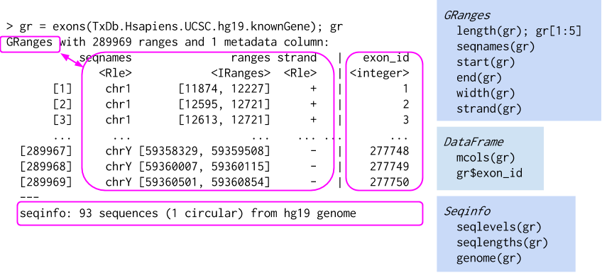
In the example above GRanges contains all exons from from hg19 UCSC database. Now to the point. What makes GRanges wholesome is all ranged-based operations they support and their speed. Practically, all operations supported by IRanges are also supported by GRanges, there is many more than mentioned before.
- Intra range transformations:
shift(),narrow(),resize(),flank() - Inter range transformations:
range(),reduce(),gaps(),disjoin() - Range-based set operations:
union(),intersect(),setdiff(),punion(),pintersect() - Coverage and slicing:
coverage(),slice() - Finding/counting overlapping ranges:
findOverlaps(),countOverlaps() - Finding the nearest range neighbor:
nearest(),precede(),follow()
plotRanges(ranges(gr))

plotRanges(ranges(reduce(gr))) # Why reduce does not work?

strand(gr) <- "*"
plotRanges(ranges(reduce(gr)))

Take your time and check out other operations on GRanges.
Challenge 2
Find genomic regions not covered by given set of
exons. Calculate coverage of those regions using ranges defined inreads.set.seed(42) # Why is it used here? exons <- GRanges(seqnames = 1, ranges = IRanges(seq(1, 100, 10), width = 9), strand = "*") seqlengths(exons) <- 100 # What does this change? reads <- GRanges(seqnames = 1, ranges = IRanges(sample.int(100, 1000, replace = TRUE), width = 2), strand = "*")Solution to challenge 2
Set seed makes sure we all have the same results, as we use sampling to create
reads. Setting lengths of chromosomes makesgaps()be aware that there is no exons with+and-strand. As allreadsare on*strand, all will fall into gaps of genomic locations on+and-strands, hence 1000.exons_gaps <- gaps(exons) countOverlaps(exons_gaps, reads)[1] 1000 1000 26 28 23 19 22 18 17 21 21 21
Now, if you have played with above operations a bit, you might have noticed that sometimes as result you will get GRangesList.
There is support in IRanges and GenomicRanges packages for Lists. GRanges inside the list have to be relative to the same genome and they have to have the same metadata columns.
grl <- split(gr, seqnames(gr))
grl
GRangesList object of length 3:
$chr1
GRanges object with 3 ranges and 2 metadata columns:
    seqnames    ranges strand |     score        GC
       <Rle> <IRanges>  <Rle> | <integer> <numeric>
  a     chr1   101-111      * |         1  1.000000
  e     chr1   105-115      * |         5  0.555556
  f     chr1   106-116      * |         6  0.444444
  -------
  seqinfo: 3 sequences from an unspecified genome; no seqlengths

$chr2
GRanges object with 3 ranges and 2 metadata columns:
    seqnames    ranges strand |     score        GC
       <Rle> <IRanges>  <Rle> | <integer> <numeric>
  b     chr2   102-112      * |         2  0.888889
  c     chr2   103-113      * |         3  0.777778
  d     chr2   104-114      * |         4  0.666667
  -------
  seqinfo: 3 sequences from an unspecified genome; no seqlengths

$chr3
GRanges object with 4 ranges and 2 metadata columns:
    seqnames    ranges strand |     score        GC
       <Rle> <IRanges>  <Rle> | <integer> <numeric>
  g     chr3   107-117      * |         7  0.333333
  h     chr3   108-118      * |         8  0.222222
  i     chr3   109-119      * |         9  0.111111
  j     chr3   110-120      * |        10  0.000000
  -------
  seqinfo: 3 sequences from an unspecified genome; no seqlengths
They still have the most important accessors.
length(grl)
[1] 3
seqnames(grl)
RleList of length 3
$chr1
factor-Rle of length 3 with 1 run
  Lengths:    3
  Values : chr1
Levels(3): chr1 chr2 chr3

$chr2
factor-Rle of length 3 with 1 run
  Lengths:    3
  Values : chr2
Levels(3): chr1 chr2 chr3

$chr3
factor-Rle of length 4 with 1 run
  Lengths:    4
  Values : chr3
Levels(3): chr1 chr2 chr3
strand(grl)
RleList of length 3
$chr1
factor-Rle of length 3 with 1 run
  Lengths: 3
  Values : *
Levels(3): + - *

$chr2
factor-Rle of length 3 with 1 run
  Lengths: 3
  Values : *
Levels(3): + - *

$chr3
factor-Rle of length 4 with 1 run
  Lengths: 4
  Values : *
Levels(3): + - *
ranges(grl)
IRangesList object of length 3:
$chr1
IRanges object with 3 ranges and 0 metadata columns:
        start       end     width
    <integer> <integer> <integer>
  a       101       111        11
  e       105       115        11
  f       106       116        11

$chr2
IRanges object with 3 ranges and 0 metadata columns:
        start       end     width
    <integer> <integer> <integer>
  b       102       112        11
  c       103       113        11
  d       104       114        11

$chr3
IRanges object with 4 ranges and 0 metadata columns:
        start       end     width
    <integer> <integer> <integer>
  g       107       117        11
  h       108       118        11
  i       109       119        11
  j       110       120        11
Metadata columns are now separated into inner (at the GRanges level) and outer (at the GRangesList level) metadata columns.
GRangesList supprt only c(), length(), names() and subsetting with [] from vector operations, but all standard list operations eg. lapply(), sapply(), endoapply(), elementNROWS(), unlist() are supported. Standard ranged operations
are also supported.
mcols(grl)$id <- paste0("ID", seq_along(grl))
mcols(grl) # outer metadata
DataFrame with 3 rows and 1 column
              id
     <character>
chr1         ID1
chr2         ID2
chr3         ID3
mcols(unlist(grl, use.names = FALSE)) # inner metadata
DataFrame with 10 rows and 2 columns
      score        GC
  <integer> <numeric>
a         1  1.000000
e         5  0.555556
f         6  0.444444
b         2  0.888889
c         3  0.777778
d         4  0.666667
g         7  0.333333
h         8  0.222222
i         9  0.111111
j        10  0.000000
With these above packages you can now manipulate your reads in many ways and calculate meaningful statistics. You know from previous lessons how to load different kinds of data, but genomic data has so many different formats. There is a lot of support from Bioconductor to load up genomic data in an easy way. Lets take a look at ShortRead package.
ShortRead
ShortRead implements sampling, iteration, and input of FASTQ files. The package includes functions for filtering and trimming reads, and for generating a quality assessment report. Data are represented as DNAStringSet-derived objects, and easily manipulated for a diversity of purposes. The package also contains legacy support for early single-end, ungapped alignment formats.
library(ShortRead)
fl <- system.file(package = "ShortRead", "extdata", "E-MTAB-1147", "ERR127302_1_subset.fastq.gz")
fq <- readFastq(fl)
fq
class: ShortReadQ
length: 20000 reads; width: 72 cycles
If you will have to parse large fastq files, it’s better to do this in streams, but it’s not our goal to create elaborate systems in this lesson. Above is simple, yet effective way of loading up data from fastq file. Notice the sample data is unpacked by the function on the fly. Yet, there is another class representing our data. There is many classes in Bioconductor, each of them has its own purpose. We will take a closer look later. You don’t need to be very intimate with every class to use it. You can always treat new, unknown classes as containers for data. You know you can always access data using slot() to force your way. You should avoid this kind of data access, unless you know exactly what are you doing.
Lets try quick exercise in quality filtering our fastq reads. First of all, without loading the file into memory we can create quality report. Run commands below. Report paths in automatically generated in your temporary directory, where you can store all kind of temporary files (function tempdir() or tempfile()). Paste path that you see into your browser to check out quality report.
qa_fq <- qa(fl)
report(qa_fq)
Lets filter out all reads with bad nucleotides.
filtered_fq <- fq[nFilter()(fq)]
Above ()() is a closure, first bracket is gonna output a function (nFilter is a function that outputs a function!), while second bracer is taking parameters for that output function. Closures are functional construct that are used in more abstract programming to create for example function factory. If you are interested in knowing more here is good resource. You can also achieve the same
goal by doing.
nF <- nFilter()
all(nF(fq) == nFilter()(fq))
[1] TRUE
Challenge 3
Lets assume we want to filter out all reads with average base quality below 30. How would you approach this problem?
Solution to challenge 3
# custom filter: mean calibrated base call quality > 30
avgQFilter <- srFilter(function(x) {
    apply(as(quality(x), "matrix"), 1, mean, na.rm = TRUE) > 30
}, name="GoodQualityBases")
fq[avgQFilter(fq)]
class: ShortReadQ length: 16736 reads; width: 72 cycles
This is an example of loading data into R and manipulating it. Now, after quality filtering lets assume that we want to process our reads a bit more. For that we need to extract sequences and operate on them. DNAStringSet is one of those classes that can hold string information, usually reads. Let’s explore them a bit more.
seq <- sread(filtered_fq)
seq
DNAStringSet object of length 19471:
        width seq
    [1]    72 GTCTGCTGTATCTGTGTCGGCTGTCTCGCGGG...CAATGAAGGCCTGGAATGTCACTACCCCCAG
    [2]    72 CTAGGGCAATCTTTGCAGCAATGAATGCCAAT...GTGGCTTTTGAGGCCAGAGCAGACCTTCGGG
    [3]    72 TGGGCTGTTCCTTCTCACTGTGGCCTGACTAA...GCATTAAGAAAGAGTCACGTTTCCCAAGTCT
    [4]    72 CTCATCCACACCTTTGGTCTTGATGGCTGTTT...AAGCATCCCGCTCAGCATCAAAGTTAGTATA
    [5]    72 GTTTGGATATATGGAGGATGGGGATTATTGCT...ATGGATAGTAATAGGGCAAGGACGCCTCCTA
    ...   ... ...
[19467]    72 GCGGGAGCGGCCAAAATGAAGTTTAATCCCTT...CGACCGAAGCAAGAATCGCAAAAGGCATTTC
[19468]    72 TTGTAATCTACTCTTGAACAAAGAATATTTAG...CAGTTTGTTGGGCAGCTAATAGTGTGAACCA
[19469]    72 TGTTGATGGTGCTGGTTACTGGGCCGTGGCTC...GGGTCCCTGCAGTTACACACAGCCCTGCCTC
[19470]    72 CGGAGGTGCAGCCCCCGCCCAAGCGGCGGCAG...ACCACACACAACCTGCCCGAGTTCATTGTGA
[19471]    72 GCAAGGGCGTCATGCTGGCCGTCAGCCAGGGC...ACCAACGGGCTCAACATCCCCAACGAGGACT
Biostrings
Biostrings - Memory efficient string containers, string matching algorithms, and other utilities, for fast manipulation of large biological sequences or sets of sequences. You probably noticed that with regular character you can’t do many operations that you would like to. The basic subsetting with the use of [] won’t do, Biostrings comes to the rescue. DNAStringSet contains DNAString objects and supports many standard character vector operations.
library(Biostrings) # Why there was no need to load it here?

length(seq)
[1] 19471
names(seq)
NULL
head(seq, 3)
DNAStringSet object of length 3:
    width seq
[1]    72 GTCTGCTGTATCTGTGTCGGCTGTCTCGCGGGAC...GTCAATGAAGGCCTGGAATGTCACTACCCCCAG
[2]    72 CTAGGGCAATCTTTGCAGCAATGAATGCCAATGG...CAGTGGCTTTTGAGGCCAGAGCAGACCTTCGGG
[3]    72 TGGGCTGTTCCTTCTCACTGTGGCCTGACTAAAA...TGGCATTAAGAAAGAGTCACGTTTCCCAAGTCT
rev(seq)
DNAStringSet object of length 19471:
        width seq
    [1]    72 GCAAGGGCGTCATGCTGGCCGTCAGCCAGGGC...ACCAACGGGCTCAACATCCCCAACGAGGACT
    [2]    72 CGGAGGTGCAGCCCCCGCCCAAGCGGCGGCAG...ACCACACACAACCTGCCCGAGTTCATTGTGA
    [3]    72 TGTTGATGGTGCTGGTTACTGGGCCGTGGCTC...GGGTCCCTGCAGTTACACACAGCCCTGCCTC
    [4]    72 TTGTAATCTACTCTTGAACAAAGAATATTTAG...CAGTTTGTTGGGCAGCTAATAGTGTGAACCA
    [5]    72 GCGGGAGCGGCCAAAATGAAGTTTAATCCCTT...CGACCGAAGCAAGAATCGCAAAAGGCATTTC
    ...   ... ...
[19467]    72 GTTTGGATATATGGAGGATGGGGATTATTGCT...ATGGATAGTAATAGGGCAAGGACGCCTCCTA
[19468]    72 CTCATCCACACCTTTGGTCTTGATGGCTGTTT...AAGCATCCCGCTCAGCATCAAAGTTAGTATA
[19469]    72 TGGGCTGTTCCTTCTCACTGTGGCCTGACTAA...GCATTAAGAAAGAGTCACGTTTCCCAAGTCT
[19470]    72 CTAGGGCAATCTTTGCAGCAATGAATGCCAAT...GTGGCTTTTGAGGCCAGAGCAGACCTTCGGG
[19471]    72 GTCTGCTGTATCTGTGTCGGCTGTCTCGCGGG...CAATGAAGGCCTGGAATGTCACTACCCCCAG
c(seq, seq)
DNAStringSet object of length 38942:
        width seq
    [1]    72 GTCTGCTGTATCTGTGTCGGCTGTCTCGCGGG...CAATGAAGGCCTGGAATGTCACTACCCCCAG
    [2]    72 CTAGGGCAATCTTTGCAGCAATGAATGCCAAT...GTGGCTTTTGAGGCCAGAGCAGACCTTCGGG
    [3]    72 TGGGCTGTTCCTTCTCACTGTGGCCTGACTAA...GCATTAAGAAAGAGTCACGTTTCCCAAGTCT
    [4]    72 CTCATCCACACCTTTGGTCTTGATGGCTGTTT...AAGCATCCCGCTCAGCATCAAAGTTAGTATA
    [5]    72 GTTTGGATATATGGAGGATGGGGATTATTGCT...ATGGATAGTAATAGGGCAAGGACGCCTCCTA
    ...   ... ...
[38938]    72 GCGGGAGCGGCCAAAATGAAGTTTAATCCCTT...CGACCGAAGCAAGAATCGCAAAAGGCATTTC
[38939]    72 TTGTAATCTACTCTTGAACAAAGAATATTTAG...CAGTTTGTTGGGCAGCTAATAGTGTGAACCA
[38940]    72 TGTTGATGGTGCTGGTTACTGGGCCGTGGCTC...GGGTCCCTGCAGTTACACACAGCCCTGCCTC
[38941]    72 CGGAGGTGCAGCCCCCGCCCAAGCGGCGGCAG...ACCACACACAACCTGCCCGAGTTCATTGTGA
[38942]    72 GCAAGGGCGTCATGCTGGCCGTCAGCCAGGGC...ACCAACGGGCTCAACATCCCCAACGAGGACT
nchar(seq)[1:10]
[1] 72 72 72 72 72 72 72 72 72 72
Also multiple summaries are possible through alphabetFrequency(), letterFrequency(), dinucleotideFrequency(). Very important for biologists is to be able to easily convert to the other strand with reverse(), complement(), reverseComplement() and translate to amino acids with translate(). Matching patterns is supported with matchPattern(), vmatchPattern() etc. Look through these possibilities.
Biostrings also has alignment options with pairwiseAlignment(). Lets align filtered reads to the first read and plot distribution of alignment scores.
aln <- pairwiseAlignment(seq, seq[1])
hist(score(aln)) # Why scores are so low?

writePairwiseAlignments(aln[1]) # Lets see first alignment.
########################################
# Program: Biostrings (version 2.58.0), a Bioconductor package
# Rundate: Thu May  6 21:51:34 2021
########################################
#=======================================
#
# Aligned_sequences: 2
# 1: P1
# 2: S1
# Matrix: NA
# Gap_penalty: 14.0
# Extend_penalty: 4.0
#
# Length: 72
# Identity:      72/72 (100.0%)
# Similarity:    NA/72 (NA%)
# Gaps:           0/72 (0.0%)
# Score: 142.6864
#
#
#=======================================

P1                 1 GTCTGCTGTATCTGTGTCGGCTGTCTCGCGGGACATGAAGTCAATGAAGG     50
                     ||||||||||||||||||||||||||||||||||||||||||||||||||
S1                 1 GTCTGCTGTATCTGTGTCGGCTGTCTCGCGGGACATGAAGTCAATGAAGG     50

P1                51 CCTGGAATGTCACTACCCCCAG     72
                     ||||||||||||||||||||||
S1                51 CCTGGAATGTCACTACCCCCAG     72


#---------------------------------------
#---------------------------------------
Challenge 4
Calculate GC content for our filtered reads. Present GC [%] information on a histogram.
Solution to challenge 4
freqs <- alphabetFrequency(seq)
GC = (freqs[,"G"] + freqs[,"C"])/rowSums(freqs)
hist(GC)

Challenge 5
Detect “ACTG” pattern in your reads and remove it from the reads.
Solution to challenge 5
midx <- vmatchPattern("ACTG", seq, fixed=FALSE)
replaceAt(seq, at = midx, value = "")
DNAStringSet object of length 19471: width seq [1] 72 GTCTGCTGTATCTGTGTCGGCTGTCTCGCGGG...CAATGAAGGCCTGGAATGTCACTACCCCCAG [2] 72 CTAGGGCAATCTTTGCAGCAATGAATGCCAAT...GTGGCTTTTGAGGCCAGAGCAGACCTTCGGG [3] 68 TGGGCTGTTCCTTCTCTGGCCTGACTAAAACC...GCATTAAGAAAGAGTCACGTTTCCCAAGTCT [4] 72 CTCATCCACACCTTTGGTCTTGATGGCTGTTT...AAGCATCCCGCTCAGCATCAAAGTTAGTATA [5] 72 GTTTGGATATATGGAGGATGGGGATTATTGCT...ATGGATAGTAATAGGGCAAGGACGCCTCCTA ... ... ... [19467] 72 GCGGGAGCGGCCAAAATGAAGTTTAATCCCTT...CGACCGAAGCAAGAATCGCAAAAGGCATTTC [19468] 72 TTGTAATCTACTCTTGAACAAAGAATATTTAG...CAGTTTGTTGGGCAGCTAATAGTGTGAACCA [19469] 68 TGTTGATGGTGCTGGTTGGCCGTGGCTCCAGG...GGGTCCCTGCAGTTACACACAGCCCTGCCTC [19470] 72 CGGAGGTGCAGCCCCCGCCCAAGCGGCGGCAG...ACCACACACAACCTGCCCGAGTTCATTGTGA [19471] 72 GCAAGGGCGTCATGCTGGCCGTCAGCCAGGGC...ACCAACGGGCTCAACATCCCCAACGAGGACT
Finally, lets save our transformed reads as “.fasta” file.
temp_file <- tempfile()
writeXStringSet(seq, temp_file)
ggbio
ggbio - package extends and specializes the grammar of graphics for biological data. The graphics are designed to answer common scientific questions, in particular those often asked of high throughput genomic data. All core Bioconductor data structures are supported, where appropriate. The package supports detailed views of particular genomic regions, as well as genome-wide overviews. Supported overviews include ideograms and grand linear views. High-level plots include sequence fragment length, edge-linked interval to data view, mismatch pileup, and several splicing summaries.
In short ggbio makes it easy to plot GRanges data, circular data, emulate genomic browser and plot ideograms! It uses the same syntax as ggplot2, it build on top of it, and figures out how to align your data for display. lets plot our ranges.
library("ggbio")
autoplot(gr)

How about some ideogram?
library("biovizBase")
hg19IdeogramCyto <- getIdeogram("hg19", cytoband = TRUE)
[1] "hg19"
plotIdeogram(hg19IdeogramCyto, "chr1")

Plot karyogram depicting information about chromosome sizes.
autoplot(hg19IdeogramCyto, layout = "karyogram", cytoband = TRUE)

Challenge 6
Plot ranges defined in
grin karyogram, but make sure to colour them by group.data(hg19Ideogram, package= "biovizBase") set.seed(42) gr <- GRanges(sample(paste0("chr", 1:13), 50, TRUE), ranges = IRanges(round(runif(50, 1, 1e8)), width = 1000)) seqlengths(gr) <- seqlengths(hg19Ideogram)[names(seqlengths(gr))] gr$group <- factor(sample(letters[1:4], 50, TRUE))Solution to challenge 6
autoplot(seqinfo(gr)) + layout_karyogram(gr, aes(fill=group, color=group))

Challenge 7
Plot the different transcripts for our genes of interest BRCA1 and NBR1.
data(genesymbol, package = "biovizBase")
library(Homo.sapiens)
Solution to challenge 7
wh <- genesymbol[c("BRCA1", "NBR1")]
wh <- range(wh, ignore.strand = TRUE)
autoplot(Homo.sapiens, which = wh)

Resources
- GenomicRanges tutorial
- browseVignettes(“GenomicRanges”)
- Closures
Key Points
Installation of most essential Bioconductor packages.
Understanding how to use Bioconductor packages.